10 million steps with R
I'm a fan of code that is computationally intense, yet very dense in terms of lines. A sort of David / Goliath kinda thing, where a few choice keystrokes can take hours to process. Additionally, when the computation can result in aesthetically pleasing output, like a 3D plot of a random walk using R's
rgl package, it's hard to resist tapping away on the keyboard for a bit.One simple and easy example of this sort of David-script is random walk data generation. With a bunch of free time this Labor-Day Weekend, I decided to take R for a long walk. Here is the code for a single step:
# Take a step, given a previous position
step <- function(old) {
  return(old + sample(-1:1,3, replace=True))
}
Since R is all about concise vector manipulation, I decided to implement the walk through iterative vector addition. Given a previous position vector, in , a random "move" vector whose components are each drawn at random from the set was created and added. To turn the steps into a walk, I decided on a number of iterations, and built up the dataset.
It was at this point that I got a real-world example of the overhead differences between raw, fixed dimension, matrices and unbounded data frames. My initial thought was to build up a data frame object from scratch, as follows:
# Walk a number of steps in R^3
walk <- function(steps) {
  path <- data.frame(x=c(0), y=c(0), z=c(0))
  for (s in 2:steps) {
    path[s,] <- step(path[s-1,])
  }
  return(path)
}
After running
walk(), as defined above and for 1,000,000 steps, my computer quickly became unresponsive. At first I thought that this was simply due to the large number of iterations, which caused each random sample call to add up. However, having just poked around in Norman Matloff's "The Art of R Programming", I remembered the discussion around R data object types.My original implementation turned out to have 2 unnecessarily taxing components. Firstly, the fact that data frames are an extension of the list class means that they inherit a bunch of unnecessary attributes for lists, such as arbitrary component types. Secondly, building up the data frame up from a small original size incurs huge cumulative costs, as with each call of
path[s,] <- step(path[s-1,])
R must copy the entire data frame, create a new one which is one row larger, and assign the new step.
To avoid both of these issues, I decided to define a correctly sized matrix object up front, and assign each step to the relevant index. The definition for
walk() then became the following:# Walk a number of steps in R^3 walk <- function(steps) { path <- matrix(nrow=steps, ncol=3) path[1,] <- c(0,0,0) for (s in 2:steps) { path[s,] <-step(path[s-1,]) } return(path) }
Now, as the appropriate amount of memory for the storage object has been declared up front, there is no need to create a new, expanded, matrix at each step. Using the
system.time() command, we can see the immense efficiency increase.> steps <- 100000 # Using an unbounded data frame > system.time(path <- walk(steps)) user system elapsed 2257.740 85.384 2337.593 # Using a defined matrix > system.time(path <- walk(steps)) user system elapsed 1.050 0.005 1.059
Having determined a speedier method, I walked R for 10 million steps and plotted the matrix using
plot3d() from rgl. Here was the path color coded chronologically, starting at the origin: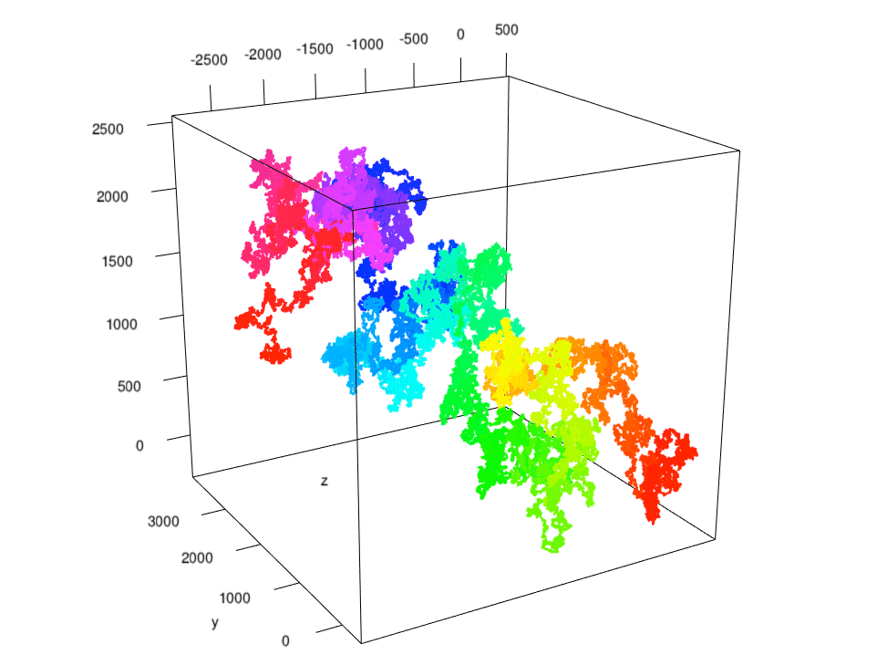
As this little project was all about making R work really hard, I decided to test the limits of my computer, as well as R's ability to deal with really big data. With the knowledge that R's maximum vector length is elements, I calculated the longest possible walk R could take. Since a matrix is just a long vector of each column sequentially concatenated, the longest 3 dimensional walk possible is steps.