Color gradients with Python
Color is one of the most powerful tools for conveying information about data. Differences in color can inspire or imply emotions (positive or negative), give a sense of magnitude (dark and dense, or light and sparse), or even hint at political persuasion (redness" and "blueness" of states on a map).
One way to convey continuous variation through colors is by using a gradient. Most graphics applications provide an easy and intuitive way to apply a gradient to a project or dataset. The ubiquitous Microsoft Excel is an easy example, with its suprisingly useful conditional formatting. Interested in how these spectra are actually constructed, I decided to try out a few ways of manually calculating color gradients using Python, given some desired input colors. Here's what I came up with!
Colors as points in 3D space
In order to "calculate" color gradients, we must first think of them as mathematical objects. Fortunately, as with everything on a computer, colors are represented numerically. This normally done as a sequence of three numbers indicating the varying amounts of Red, Green, and Blue, either in decimal tuple (70,130,180) or hex triplet (#4682B4) form (both examples given represent steel blue, the main color used on this site). This means we can think of a color abstractly as a vector () in three dimensional space.
Practically, within Python, I sometimes want to pass these colors / vectors as hex triplet strings and other times as RGB tuples (implemented as lists to allow mutable components). Here are two basic functions I ended up using for converting accross formats:
def hex_to_RGB(hex):
  ''' "#FFFFFF" -> [255,255,255] '''
  # Pass 16 to the integer function for change of base
  return [int(hex[i:i+2], 16) for i in range(1,6,2)]


def RGB_to_hex(RGB):
  ''' [255,255,255] -> "#FFFFFF" '''
  # Components need to be integers for hex to make sense
  RGB = [int(x) for x in RGB]
  return "#"+"".join(["0{0:x}".format(v) if v < 16 else
            "{0:x}".format(v) for v in RGB])
With colors as vectors, gradients can then be thought of as functions of colors, with each component of evolving for different input values.
Linear Gradients and Linear Interpolation
The simplest type of gradient we can have between two colors is a linear gradient. As the name suggests, this gradient is a function representing a line between the two input colors. The following is an example of a gradient that varies from black to gray to white, taking in a value of which specifies how far along the gradient the desired output color should be:
In Python, I implemented this as a function which, given two hex imputs, returns a dictionary containing a desired number of hex colors evenly spaced between them as well as the corresponding RGB decimal components as individual series.
def color_dict(gradient):
  ''' Takes in a list of RGB sub-lists and returns dictionary of
    colors in RGB and hex form for use in a graphing function
    defined later on '''
  return {"hex":[RGB_to_hex(RGB) for RGB in gradient],
      "r":[RGB[0] for RGB in gradient],
      "g":[RGB[1] for RGB in gradient],
      "b":[RGB[2] for RGB in gradient]}


def linear_gradient(start_hex, finish_hex="#FFFFFF", n=10):
  ''' returns a gradient list of (n) colors between
    two hex colors. start_hex and finish_hex
    should be the full six-digit color string,
    inlcuding the number sign ("#FFFFFF") '''
  # Starting and ending colors in RGB form
  s = hex_to_RGB(start_hex)
  f = hex_to_RGB(finish_hex)
  # Initilize a list of the output colors with the starting color
  RGB_list = [s]
  # Calcuate a color at each evenly spaced value of t from 1 to n
  for t in range(1, n):
    # Interpolate RGB vector for color at the current value of t
    curr_vector = [
      int(s[j] + (float(t)/(n-1))*(f[j]-s[j]))
      for j in range(3)
    ]
    # Add it to our list of output colors
    RGB_list.append(curr_vector)

  return color_dict(RGB_list)
Outputting the RGB components as points in 3D space, and coloring the points with their corresponding hex notation gives us something like this (gradient ranges from
#4682B4 to #FFB347):
Multiple Linear Gradients ⇒ Polylinear Interpolation
While one linear gradient is fun, multiple linear gradients are more fun. Taking
linear_gradient() and wrapping it in a function which takes in a series of colors, we get the following gradient function (I've also included a function for generating random hex colors, so I don't have to spend time choosing examples):from numpy import random as rnd def rand_hex_color(num=1): ''' Generate random hex colors, default is one, returning a string. If num is greater than 1, an array of strings is returned. ''' colors = [ RGB_to_hex([x*255 for x in rnd.rand(3)]) for i in range(num) ] if num == 1: return colors[0] else: return colors def polylinear_gradient(colors, n): ''' returns a list of colors forming linear gradients between all sequential pairs of colors. "n" specifies the total number of desired output colors ''' # The number of colors per individual linear gradient n_out = int(float(n) / (len(colors) - 1)) # returns dictionary defined by color_dict() gradient_dict = linear_gradient(colors[0], colors[1], n_out) if len(colors) > 1: for col in range(1, len(colors) - 1): next = linear_gradient(colors[col], colors[col+1], n_out) for k in ("hex", "r", "g", "b"): # Exclude first point to avoid duplicates gradient_dict[k] += next[k][1:] return gradient_dict
This means we can pick a few colors we want to our data to "evolve through", and get back a series of corresponding interpolated colors. Below is an example of linear gradients running through 5 different random colors, with 50 total interpolated colors.
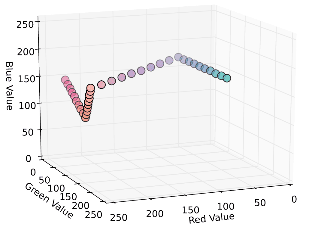
While this serves the purpose of providing a gradient through multiple colors, it does so in a sort of jagged, inelegant way. What would be better is a smooth evolution accross the colors, with each input color providing various amounts of influence as we move through the gradient. For this, we can turn to Bezier Curves.
Nonlinear Gradients: Bezier Interpolation
While I will leave the denser mathematical description of Bezier Curves to Wikipedia and this guys awesome notes (PDF), they can easily be used to provide smooth gradients through various control colors (corresponding to Bezier control points). To implement Bezier gradients in Python, I took advantage of the following polynomial notation for n-degree Bezier curves () through control colors ():
The Python implementation of this took the following form, with a helper function for the Bernstein coefficient. I also chose to memoize the factorial function, it can be expected that the inputs will be consistantly similar due to its range consisting of integers in and its recursive implementation.
# Value cache
fact_cache = {}
def fact(n):
  ''' Memoized factorial function '''
  try:
    return fact_cache[n]
  except(KeyError):
    if n == 1 or n == 0:
      result = 1
    else:
      result = n*fact(n-1)
    fact_cache[n] = result
    return result


def bernstein(t,n,i):
  ''' Bernstein coefficient '''
  binom = fact(n)/float(fact(i)*fact(n - i))
  return binom*((1-t)**(n-i))*(t**i)


def bezier_gradient(colors, n_out=100):
  ''' Returns a "bezier gradient" dictionary
      using a given list of colors as control
      points. Dictionary also contains control
      colors/points. '''
  # RGB vectors for each color, use as control points
  RGB_list = [hex_to_RGB(color) for color in colors]
  n = len(RGB_list) - 1

  def bezier_interp(t):
    ''' Define an interpolation function
        for this specific curve'''
    # List of all summands
    summands = [
      map(lambda x: int(bernstein(t,n,i)*x), c)
      for i, c in enumerate(RGB_list)
    ]
    # Output color
    out = [0,0,0]
    # Add components of each summand together
    for vector in summands:
      for c in range(3):
        out[c] += vector[c]

    return out

  gradient = [
    bezier_interp(float(t)/(n_out-1))
    for t in range(n_out)
  ]
  # Return all points requested for gradient
  return {
    "gradient": color_dict(gradient),
    "control": color_dict(RGB_list)
  }
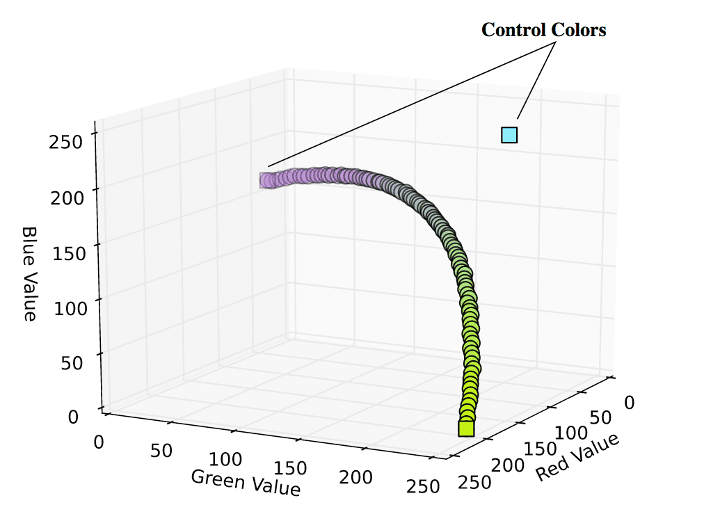
The result of this more technical gradient calculation is a smoother range, influenced by its given control colors. The following example takes in 3 control colors, but the above function can handle Bezier Curves of arbitrary degree.
Matplotlib Plotting Stuff
Finally, here is the code I used to plot the points generated by the various gradient functions. All that is required is the matplotlib package.
from mpl_toolkits.mplot3d import Axes3D
import matplotlib.pyplot as plt

def plot_gradient_series(color_dict, filename,
             pointsize=100, control_points=None):
  ''' Take a dictionary containing the color
      gradient in RBG and hex form and plot
      it to a 3D matplotlib device '''

  fig = plt.figure()
  ax = fig.add_subplot(111, projection='3d')
  xcol = color_dict["r"]
  ycol = color_dict["g"]
  zcol = color_dict["b"]

  # We can pass a vector of colors
  # corresponding to each point
  ax.scatter(xcol, ycol, zcol,
             c=color_dict["hex"], s=pointsize)

  # If bezier control points passed to function,
  # plot along with curve
  if control_points != None:
    xcntl = control_points["r"]
    ycntl = control_points["g"]
    zcntl = control_points["b"]
    ax.scatter( xcntl, ycntl, zcntl,
                c=control_points["hex"],
                s=pointsize, marker='s')

  ax.set_xlabel('Red Value')
  ax.set_ylabel('Green Value')
  ax.set_zlabel('Blue Value')
  ax.set_zlim3d(0,255)
  plt.ylim(0,255)
  plt.xlim(0,255)

  # Save two views of each plot
  ax.view_init(elev=15, azim=68)
  plt.savefig(filename + ".svg")
  ax.view_init(elev=15, azim=28)
  plt.savefig(filename + "_view_2.svg")

  # Show plot for testing
  plt.show()