Dynamic reports with "StaTeX"
As a big fan of LaTeX and daily slave to Stata, I've put a little thought into finding easy ways to bring the aesthetics and clarity of the former to the output of the later. In particular, there are two great Stata modules (
estout and texdoc, both available through SSC) which, when combined with Stata's shell interface, make it easy to compile professional and organized output. In this post, I present a sample (OSX oriented) code structure for a single .do file which conducts analysis, generates TeX source code, and then compiles that source to pdf.
Recently, I've been working on a few projects for Urban which involve constructing large multivariate models. The process includes constant tweaking of various parameters such as sample restrictions and control variables. As a project progresses, keeping track of these changes can be difficult. Keeping track of the evolving components and outcomes of a model as it is modified can make the construction process simpler. As shown here, this can be easily done by creating a LaTeX output document upon each run of the analysis do file.
Producing nice-looking LaTeX tables with Stata
One way to concisely illustrate coefficient and standard error changes during model construction is through a table like this :
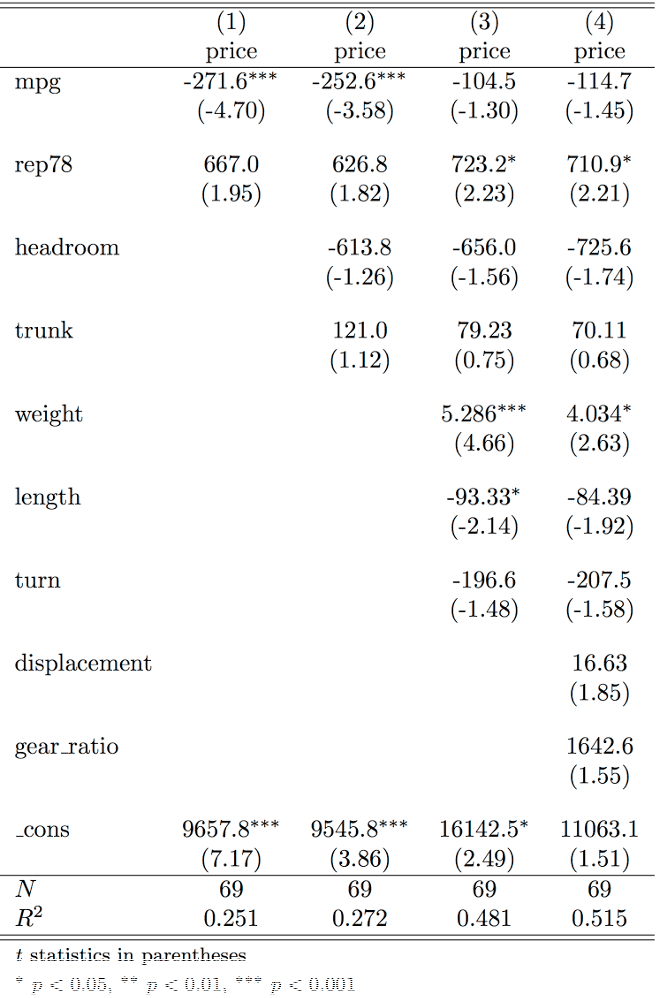
which shows a few simple linear regressions of automobile price on various controls, and is produced using the
tabular environment found in LaTeX. While the end product as shown above gives you a clear idea of how the influence of independent variables change when others are included, producing this table is normally an involved process.As the nifty little graphic below abstractly illustrates, producing, inserting, and compiling LaTeX tables is usually a 3 step process. First, analysis is conducted and the corresponding TeX source code for the table is generated. This has fortunately been made simple through packages like
estout, which allows for easy production of professional looking tables. For an example of how to produce these tables, see the Stata source for the table produced above.However, as each call of
esttab only produces the stand alone table, documents with multiple models or graphics need a master LaTeX document, which contains the preamble, and the required \begin{document} and \end{document} statements. The second step below illustrates the necessity of importing the individual analytical graphics into a master source file, which then must be compiled using pdflatex or some variant (the third and final step)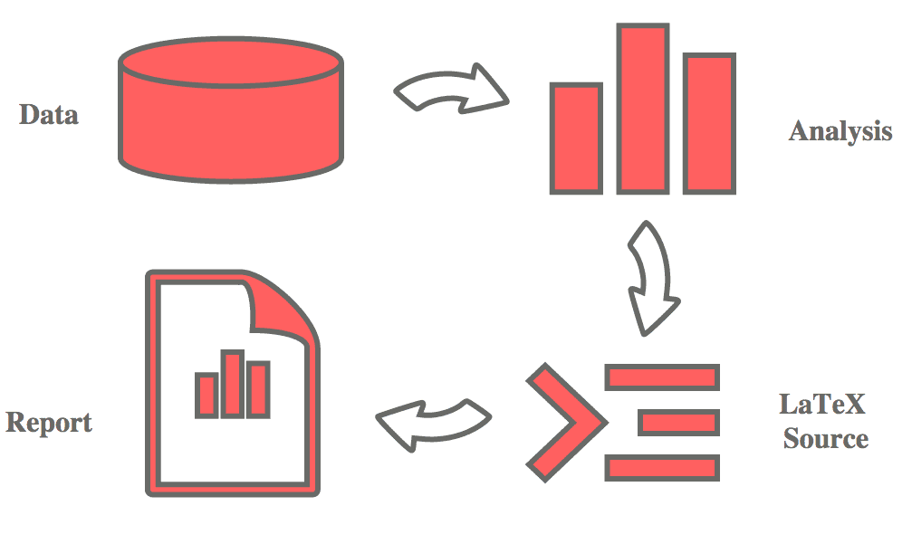
After using
esttab for a while, I began to find this multi-stage task a little bit of a chore, and set out to learn how best to streamline the process. I first looked for a method to eliminate the need for a separate master LaTeX source file.Cutting out the middle man: writing complete LaTeX documents within Stata
To streamline the report generation process, the whole LaTeX document would ideally be created from within Stata. This was achieved through the excellent
texdoc package, which allows for inline TeX syntax within Stata .do files, similar to a reverse Sweave (R's literate programming extension). This meant that the necessary preamble found in all LaTeX documents could be neatly inserted into the start of the corresponding analysis .do file.For those familiar with TeX syntax,
texdoc is pretty simple to use. Here is an example beginning to a .do file using texdoc:/* Initialize the TeX master source document */ texdoc init test.tex, replace /* Begin stream of LaTeX code */ /*tex \documentclass{article} \usepackage[top=1in, left=1in]{geometry} \usepackage{stata, hyperref, fancyhdr} \setlength\parindent{0pt} \pagestyle{fancyplain} % (LaTeX Comment) Define new command to add % tables with linked header (using fancyhdr) \newcommand{\addtab}[1]{ \lhead{} \rhead{} \chead{\hyperlink{top}{Back To Top}} \newpage \begin{table} \caption{{"{#1}"}} \centering \input{{"{#1}"}} \end{table} } \begin{document} \thispagestyle{empty} % Manual title (with a link target) \hypertarget{top}{\textbf{\Large Model Building Example}} \vspace{10pt} Author: Ben Southgate tex*/ /* End Stream of LaTeX */ /* Use Stata global macros to record run time/date */ tex Compiled: $S_TIME, on $S_DATE tex \vspace{20pt}
As shown above,
texdoc works by writing a LaTeX document line by line, simply adding tex before any actual TeX commands. You can also write a long stream of TeX between /*tex ... tex*/ delimiters, though the file must then be run with texdoc do filename.do. This means that needed LaTeX packages and their parameters can be set with a few calls at the beginning of the do file. One important LaTeX package called above is the "Stata" package, which allows inclusion of Stata's own markup language (SMCL) within TeX documents for presentation of console output in Stata Journal format.Additionally, as shown in the last code fragment, the Stata date macros
$S_DATE and $S_TIME can be called within the tex calls. While model building, I used these to keep track of the run time within the LaTeX document. As elements stored in Stata global and local macros are realized before outputting to the TeX document, they can be used as normal within tex commands.Next, with the master LaTeX document initialized, actual analysis and table generation could begin. For example, lets note some sample restrictions in our report and then recreate the table shown above.
/* Load system data */
sysuse auto, clear

/* Clear any current estimation storage macros */
eststo clear

tex
tex \textbf{\large Sample Restrictions}
/*  Comments and code after this point will be ouput to
    LaTeX document in full */
texdoc stlog

/* Sample Restrictions */
keep if (               ///
    weight < 4500 &     ///
    price  < 10000      ///
)

texdoc stlog close
/* Now stata code is no longer output */

/* List all the LaTeX tables */
tex \listoftables


/* Run regressions and store results */
eststo: reg price mpg rep78
eststo: reg price mpg rep78 head trunk
eststo: reg price mpg rep78 head trunk weight len turn
eststo: reg price mpg rep78 head trunk weight len turn disp gear

/* Create LaTeX table to be included in a separate document */
esttab using ModelBuild.tex, tex r2 replace

tex \addtab{ModelBuild}

tex \end{document}
texdoc close // Close the LaTeX document, which can now be compiled
In the code above, the command
texdoc stlog initiates verbatim recording of Stata commands and their output, writing it all to the LaTeX document. This can be useful, as shown above, to keep track of what sample restrictions went in to this particular run of the models. In the final LaTeX document, the Stata package is required to render anything recorded with stlog.Additionally, the command
tex \listoffigures creates a hyper-linked list of figures, letting you zip around the document even if there are a large number of models or charts.The final command,
tex \addtab{ModelBuild}, calls the LaTeX function defined above which inserts the table into the master document, and creates a hyper-linked header allowing for easy document navigation back to the top. I found this useful when I had 50+ charts in one document.Shell within Stata: Compiling the LaTeX output from the .do file
Now that we have a LaTeX document ready to be compiled, all we need to do is run it through pdflatex. Luckily, Stata provides built-in commands to interface with the OS Shell, allowing LaTeX compiling without leaving the .do file. Below, I've provided a few commands for doing precisely this in OSX 10.8, with MacTeX installed:
/* Stop LaTeX output from requiring manual continuation */
set more off

/* Create "filename-friendly" strings indicating the runtime */
local date = subinstr("$S_DATE _"," ","",.)
local time = subinstr("$S_TIME",":","_",.)

/*  Execulte shell commands to compile and open LaTeX output,
    move the pdf to the output folder, and remove latex junk.

    Note: pdflatex is run twice to allow \listoftables links to work
*/
shell /usr/texbin/pdflatex test.tex
shell /usr/texbin/pdflatex test.tex
shell mv test.pdf /output/test`date'`time'.pdf
shell open /output/test`date'`time'.pdf
shell rm *test*
As is evident above, normal Unix and Mac commands work fine, though the
$PATH is not available so you'll have to indicate where pdflatex is installed. A further note to those interested in replicating this, you will need to install the Stata journal package and its corresponding LaTeX files. This can be done by entering findit sjlatex in Stata and following the directions.